Introduction: Business Problem
I used to work in the mortgage industry processing and closing residential loans. At that time, I did not know some of the factors that influence house prices or how to determine the correlation between the housing features and price. I express particular interest in this topic because of my background. Studying data science with Coursera and IBM provides me with some knowledge, insight, and a curious mind to go little deeper and determine what features buyers are interested in and willing to pay more for them.
Aside from my personal interest in this topic, the target audience I believe the outcome of this project will benefit may be mortgage or lending companies, buyers, individual sellers, real estate brokers, and independent contractors (building, remodeling houses) in the Minneapolis housing market. The results of this project, I hope, will help these interested parties better estimate the house prices with certain features.
In this project, I explore the determinants of house prices in the Minneapolis neighborhood housing market. What are the features in a house that interested parties are looking for and willing to pay more? What features have a strong correlation with house prices? These questions and more are examined further in this project. Not all features studied in this project have equal or strong correlation to the price. In other words, correlation between housing features varies as noted in the analysis section of this report.
Methodology
As noted above, the focus of this project is to examine the effect of selected features on residential house prices in the Minneapolis neighborhood market. Luckily, the dataset is organized by the city of Minneapolis and freely available at the Open Minneapolis website. On the website, the data is available from 2017 to 2020. I chose 2019 because I thought is most recent and complete. The dataset in csv file is downloaded and has 130,915 rows and fifty-three columns. The column name “property type” has residential, double bungalow, triplex, apartment, commercial, condominiums, vacant land, cooperative, etc., property types. The focus of this report is on residential property types as such other property types are dropped from the study. After initial data wrangling, the data frame has 75,328 rows and twenty-one columns remaining.
Out of the fifty-three columns in the data frame, I choose the following columns for processing:
| ZIPCODE | Postal code |
| FORMATTED_ADDRESS | Full mailing address |
| PARCEL_AREA_SQFT | Land area of parcel in square feet |
| X | coordinate of parcel centroid (uses NAD 83 HARN Hennepin County coordinate system) |
| Y | coordinate of parcel centroid (uses NAD 83 HARN Hennepin County coordinate system) |
| PROPERTY_TYPE | Type of property |
| NEIGHBORHOOD | Name of neighborhood the property is in |
| LANDVALUE | Property’s assessed land value as of January 2 of its assessment year |
| BUILDINGVALUE | Property’s assessed building value as of January 2 of its assessment year |
| TOTALVALUE | Property’s total assessed value as of January 2 of its assessment year |
| BELOWGROUNDAREA | Total square footage below grade |
| ABOVEGROUNDAREA | Total square footage above grade |
| NUM_STORIES | Number of stories in building |
| GARAGE_PRESENT | Indicates whether property has a garage |
| PRIMARYHEATING | Primary type of heating in building |
| CONSTRUCTIONTYPE | Style of construction |
| EXTERIORTYPE | Exterior finish of building |
| ROOF | Style of roof |
| FIREPLACES | Number of fireplaces |
| BATHROOMS | Number of bathrooms |
| BEDROOMS | Number of bedrooms |
In the analysis section, I used box plots to determine the relationship between the object data types such as primary heating, exterior type, construction type, and roof to provide visual depiction of the relationships. Some integer and float data types are depicted visually for those who may not be familiar with numbers in regression analysis. Foursquare API is used as a requirement for this project to construct a URL, search for venues, request for venues, and explore the geographical location in the city of Minneapolis, Minnesota. Folium, the visualization library, is used to visualize the results. This dataset, Minneapolis Neighborhoods, was downloaded from Open Minneapolis site.
Analysis
As mentioned above, box plots are used to visualize the relationships between the object data types and the building value or price. I take advantage of one of the benefits of box plots, i.e., comparing the distribution of multiple datasets. Look at the box plot below displaying the distribution of multiple heating units that can be installed in houses in Minneapolis. From the box plots below, it’s clear that the distribution of building value in all the categories under primary heating, exterior type, construction type, and roof are distinct enough to be considered as potential predictors of building value. The tables below each box plot show the average building price for each categorical variable. Interested parties do not have to be data scientists to compare the visual and numerical representation of the data.

| PRIMARYHEATING | BUILDINGVALUE | |
| 0 | ELECTRIC | 148578.625954 |
| 1 | FORCED AIR | 226756.243957 |
| 2 | GEOTHERMAL | 841377.500000 |
| 3 | GRAVITY | 161065.417256 |
| 4 | HOT WATER | 301815.756115 |
| 5 | RADIANT FLOOR | 502555.555556 |
| 6 | STEAM | 483065.034965 |
| 7 | UNIT HEATERS | 121676.555024 |

| EXTERIORTYPE | BUILDINGVALUE | |
| 0 | BRICK | 406892.531705 |
| 1 | CONCRETE | 420098.305085 |
| 2 | FIBER CEMENT BOARD | 410577.536946 |
| 3 | METAL/VINYL | 205204.886799 |
| 4 | OTHER | 180485.735115 |
| 5 | STONE | 563175.229358 |
| 6 | STUCCO | 251052.487628 |
| 7 | WOOD | 250461.232968 |

| CONSTRUCTIONTYPE | BUILDINGVALUE | |
| 0 | BRICK & MILL | 444228.421053 |
| 1 | CONCRETE | 561040.000000 |
| 2 | METAL | 376200.000000 |
| 3 | OTHER | 361300.000000 |
| 4 | REINFORCED CONCRETE | 660821.428571 |
| 5 | STEEL FRAME | 367929.411765 |
| 6 | WOOD FRAME | 242848.606534 |
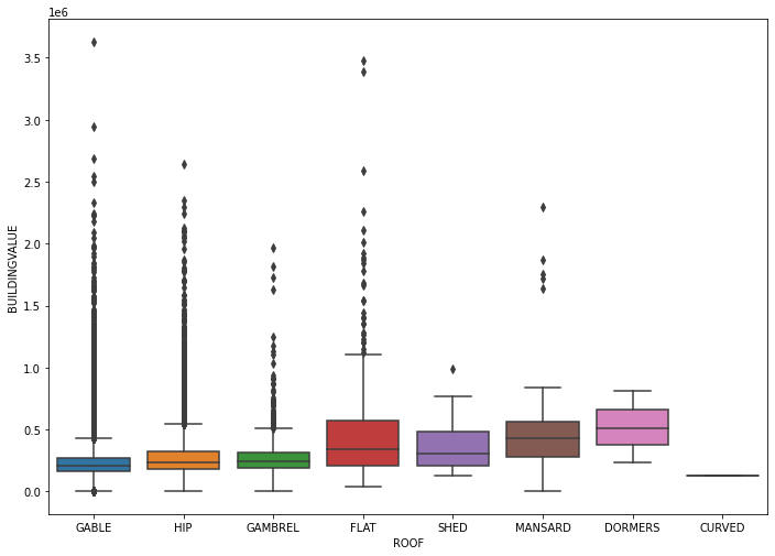
| ROOF | BUILDINGVALUE | |
| 0 | CURVED | 131200.000000 |
| 1 | DORMERS | 517566.666667 |
| 2 | FLAT | 487314.285714 |
| 3 | GABLE | 234420.681748 |
| 4 | GAMBREL | 272766.173362 |
| 5 | HIP | 280136.134454 |
| 6 | MANSARD | 506101.265823 |
| 7 | SHED | 380957.142857 |
Linear Regression

Results and Discussion
The analysis of the house data, using the object variables, reveals noticeable increase in average building value for some variables and lower average price for others. For example, the primary heating has an average building value of $841,377.50 for a house with Geothermal heating unit and $121676.55 for a house fitted with Unit heaters at the lower end. These clear shows that the determinants chosen in this study affect the house prices in the Minneapolis neighborhoods area. Interested parties are therefore presented with a choice about what material to use if they want to increase the value of the house. It may be cost variables that affect the value of a house or other factors. Whatever the reason, there are clear variations in values of houses fitted with different units.
While searching and replacing missing values, I noticed that the most frequent categorical variables in their respective categories are not those that add highest average value to the house. In other words, the materials most used by builders ranked at the very bottom with respect to increased value of the house. For example, forced air ranked fifth out of seven, wood frame sixth out of six, stucco fifth out of seven, and gable ranked sixth out of seven categories. For better visualization and comprehension of these observations, please refer to the categorical figures and their respective tables above. Grouping the construction type and roof type, the combination of the reinforced concrete and flat roof type is the most expensive ($946,416.70).
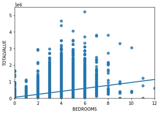
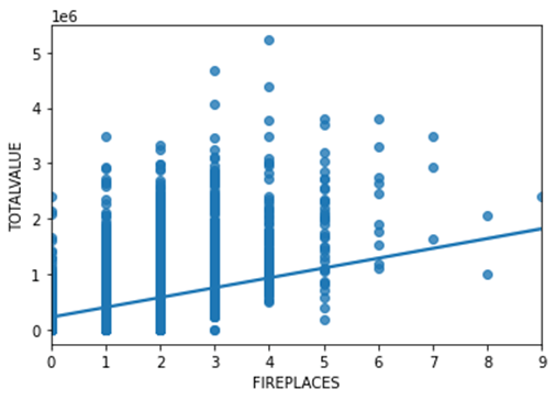
Applying the Pearson Correlation Coefficient and P-value, I found the correlation between the number of bedrooms, bathrooms, and fireplace to be statistically significant though, the linear relationships in all three of them are moderately strong. These results are consistent with statistical table on the Jupyter notebook.
| Pearson Correlation Coefficient | P-value | |
| Bedrooms | 0.3810128178868299 | 0.0 |
| Bathrooms | 0.6622152395520273 | 0.0 |
| Fireplaces | 0.5727427014314311 | 0.0 |
Foursquare API is used to request interesting venues in Minneapolis neighborhoods. Some venues are found and listed on the map. When I run k-means to cluster the neighborhoods, I am surprised to find only 1 cluster in Minneapolis neighborhoods. I started with k=5 to k=2 getting error in all of them. When I set k=1, it works simply fine with one dot on the map.
In model evaluation, the results are both visualized and measured quantitatively to determine the accuracy of the model. In this study, I used the R^2 to determine how accurate the models are. R square or the coefficient of determination, is a measure to show how close the data is to the fitted regression line. The value of the R^2 is the percentage of variation of the response variable (y) that is explained by a linear model. For linear regression, ridge regression, and second-degree polynomial I used the total value (which include the land and building values) to calculate the R^2 values. In second-degree polynomial, both the training data and testing data are used to calculate R^2 values and the results are 0.7847696530237769 and 0.7713001435645377, respectively. I can now say that ~78.48% of the Variation of total value is explained by this polynomial fit. The ridge regression on trained data has R^2 of 0.710036153823197 and simple linear regression is 0.6239123580483767. Please refer to the code on Jupyter Notebook for complete results.
Conclusion
In conclusion, the determinants studied in this project have some correlation to the residential properties at various levels. In the categorical variables section, for example, I found a noticeable increase in average house values with certain categorical variables. For example, houses with reinforced concrete have a higher average value than other categorical variables in the same category. Finally, I observed that the most used variables under the primary heating, construction type, exterior type, and the roof are the least valuable in terms of the average building values. This brings us to the question that may be explored further in future research. And that is, why are the variables that least increase the average value of a house the most used by builders or owners?
